8 Site assessment

8.1 Secondary research

Chances are, you already know where you’ll be conducting your walkability assessment. This could be your neighborhood, a section of an area you visit often, or even a place you’ve never been to. If you have already narrowed down such a region, 8.1.2 shows you how to identify important and busy streets for your audit. 8.1 shows you how to get information about your site’s population, which can help you understand the region’s demographics.

8.1.1 Understanding the population

In 6, we discussed the importance of adding a socio-economic layer of context to our assessments. TLDR; understanding your demographic, income levels, and social makeup can help you show who is being excluded and design your solutions more inclusively. We can use a variety of data sources to view information about the population. I discuss some ways to use this data to identify segregation within areas in Section 17.2

Census data

The last general census in India was conducted in 2011. While outdated by almost all counts, this data remains the only comprehensive source of information at a country-wide level. The highest resolution (the level of detail) at which this data is available is at a city’s ward level. If you live in any of the large metro cities, this might already be available through OpenCity. Some states and government bodies have also opened their GIS servers for access, a full list of which you can find here. For smaller cities, the compiled population information by (balk2019?) for the entire country from a variety of sources can be downloaded in the form of CSV and GeoTIFF files.

Global Human Settlement Layer

The Global Human Settlement Layer (GHSL) by the Joint Research Centre provides high-resolution population estimates for nearly every country. This can be downloaded for various years (in my experience, the 2015 dataset works well) and for your specific region of interest through the website’s interactive map.

The GHSL dataset is commonly used for estimating the population, whereas other datasets might be hard to get. The data is provided in raster format, where each pixel represents the number of people at that point. You can easily visualize this in software like QGIS. An excellent project that makes it available to explore only is Tom Forth’s Population around a point.

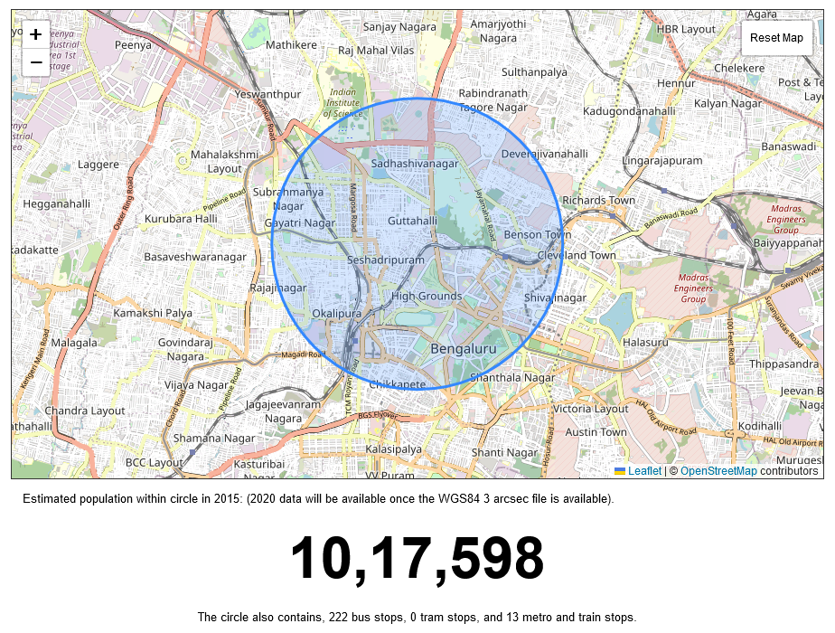
Figure 8.1: The global coverage makes GHSL a very useful source of data on population.

8.1.2 Understanding the space

You have your region, and you know something about your population. Now how would you decide which streets to audit? Space Syntax Analysis (SSA) can help!

Space syntax analysis is a method of analyzing and understanding the spatial configuration of built environments developed by University College London (UCL) researchers in the 1970s and 1980s.

The basic premise of space syntax analysis is that how buildings and cities are configured spatially can significantly impact how people use and interact with those spaces. By analyzing the spatial relationships between different parts of a built environment, space syntax analysis can help reveal movement patterns, interaction, and social activity (van Nes and Yamu 2021). This can be done using street networks from OpenStreetMap and DepthMapX, a software dedicated to such analysis.

8.1.3 Components of Space Syntax Analysis

There are three measures that this method will provide you with. In extremely simple, intuitive terms, these are:

1. Choice: Choice is a way to measure how likely a street or road segment is to be used by people traveling between different parts of a system. For example, imagine a city and all the different routes people could take to get from one place to another. Choice measures how often a particular street segment is used on the shortest path between any two locations in the system. A high choice value means that many people are likely to use that street segment, while a low choice value means fewer people are likely to use it. So, the choice measures how important a street segment is for connecting different system parts (Hillier and Hanson 1984).

2. Integration: Integration is a way to measure how close or connected one place is to all the other places in a system. For example, think of a city and its different neighborhoods. Integration measures how easy it is to get from one area to another. The higher the integration, the more connected the neighborhoods are and the easier it is to move around (Hillier and Hanson 1984).

We can use these measures to extrapolate many insights from quantitative data in the form of street networks and build a model for understanding the space. The theory also proposes that the street network adapts and changes over time to intensify local connections, which leads to more efficient movement patterns and porous structures. Essentially, SSA describes how the layout of the street network shapes the development of urban centers and how the evolution of the street network over time influences the formation and location of centers within the urban settlement layout as a whole.

8.1.4 Using DepthmapX for SSA

So you’ve chosen your area to audit, but you want to maximize your resources and time and start by auditing the most important streets in the region. If you know the neighborhood, you already know what to do. If not, the choice measure can help you provide a starting point.

First, get the following things ready before moving ahead:

1. Download DepthmapX: You can find the relevant copy for your operating system here.

2. Download your region’s OSM street network: Trim the network to your region of interest so you can process the data faster.

3. Fire up QGIS: We’ll use this to convert our street files into an appropriate format for use in DepthMapX and then bring it back here for polishing touches after analysis.

Let’s get started!

Step 1. Convert your street network into .mif

.mif stands for a MapInfo file, which is a type of digital file that contains information about a map. It is like a virtual version of a paper map that can be opened on a computer. It contains data about different features on the map, such as roads, buildings, and rivers; basically everything you’ll need about your street network to pull it into DepthmapX.

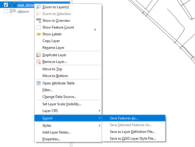
You can do this by right clicking on your street layer and going to Export > Save Features As and selecting .mif from the export dialog box.

8.1.4.1 Step 2. Prepare it in DepthMapX {.unnumbered}

Open your copy of DepthMapX and create a new project by going to File > New. We can now import our map by going to Map > Import.

What you should now see is a map with all streets with different colors. Each part of a street that is a different color is a segment. Right now, DepthMapX does not know how much each segment measures. To do that, go to Tools > Convert Active Map and choose Segment Map from the dialog that opens.

Once you click OK, your map should process and be done fairly quickly.

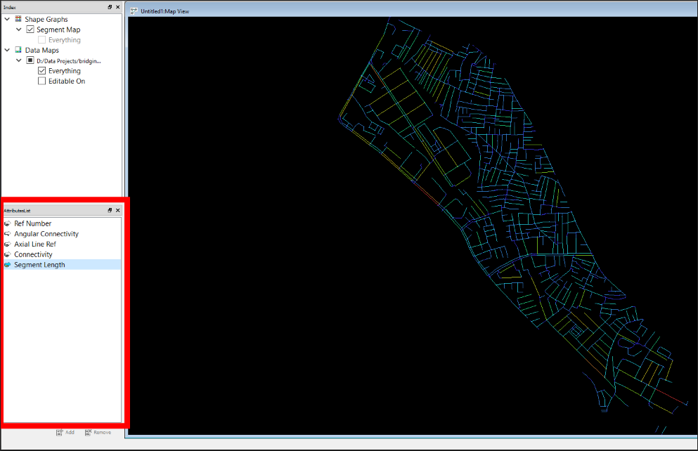
In your Attributes List pane on the left-hand side, you can click on various layers and watch the map update in colors. Here’s what is important for you:

1. Ref Number is a unique ID for each segment.

2. Angular Connectivity is a way of measuring the degree of connectivity between different segments of a street network. It is calculated by adding up the cumulative turn angles from a root segment to all other segments in the network. Essentially, it measures the overall angle of turns that must be made when traveling from the root segment to other segments, which can indicate how direct or indirect the route is.

   For example, if you have a network of streets and you want to travel from point A to point B, segment angular connectivity would measure the total angle of turns you would need to make along the way. A high segment angular connectivity would mean that there are many turns along the way, while a low segment angular connectivity would indicate a more direct route. This metric can be useful in analyzing the accessibility and ease of movement within a street network.

3. Connectivity is a measure of how many other spaces are directly connected to a given space in a system.

   For example, in a street network, connectivity measures the number of streets that intersect with a particular street or node, which can affect how easily people can move between different areas of the city. Higher connectivity generally means that there are more direct routes between spaces, which can make movement more efficient and promote social interaction.

4. Segment Length, as the name implies, color codes the parts of the street network that have similar lengths.

Step 3. Run Segment Analysis

We need to find out which roads are the most important, or the busiest, in this region. Go to Tools > Segment > Run Angular Segment Analysis.

This should bring up a dialog box that looks something like Figure (ref?)(fig:segment-analysis). For best results, here are the recommended settings and what they mean:

1. Tulip Bins refers to how accurate (hence slower) or less accurate (faster) the analysis should be. Any value around 500 is good enough.

2. Include choice should be ticked because that is the measure we are interested in.

3. Radius Type should be metric because we’re measuring values in meters.

4. Radii refers to the distances or areas surrounding a central point, also known as a root space. This is how much area can be covered with ease for different types of mobility. Generally, it is 400m for pedestrians, 800m for cyclists and we’ll keep the rest n because this is all we’re interested in at the moment.

5. Weighted measures should be ticked, and set to Segment Length because we want that metric to be used to measure all these values.

Once you’ve done this, run and wait!

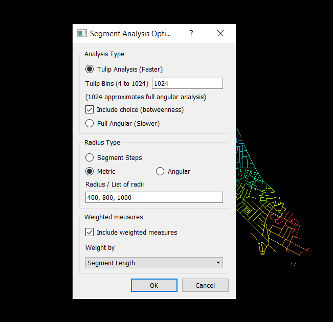
Figure 8.2:

If all goes well, your Attributes List pane should be filled with new layers. Play around with them, what do you understand?

The layer we’re interested in should be named T1024 Choice (or whatever number you set for tulip bins). Once you click on it, most of the colors should disappear and you should have a few streets being highlighted, as shown in Map 8.3.

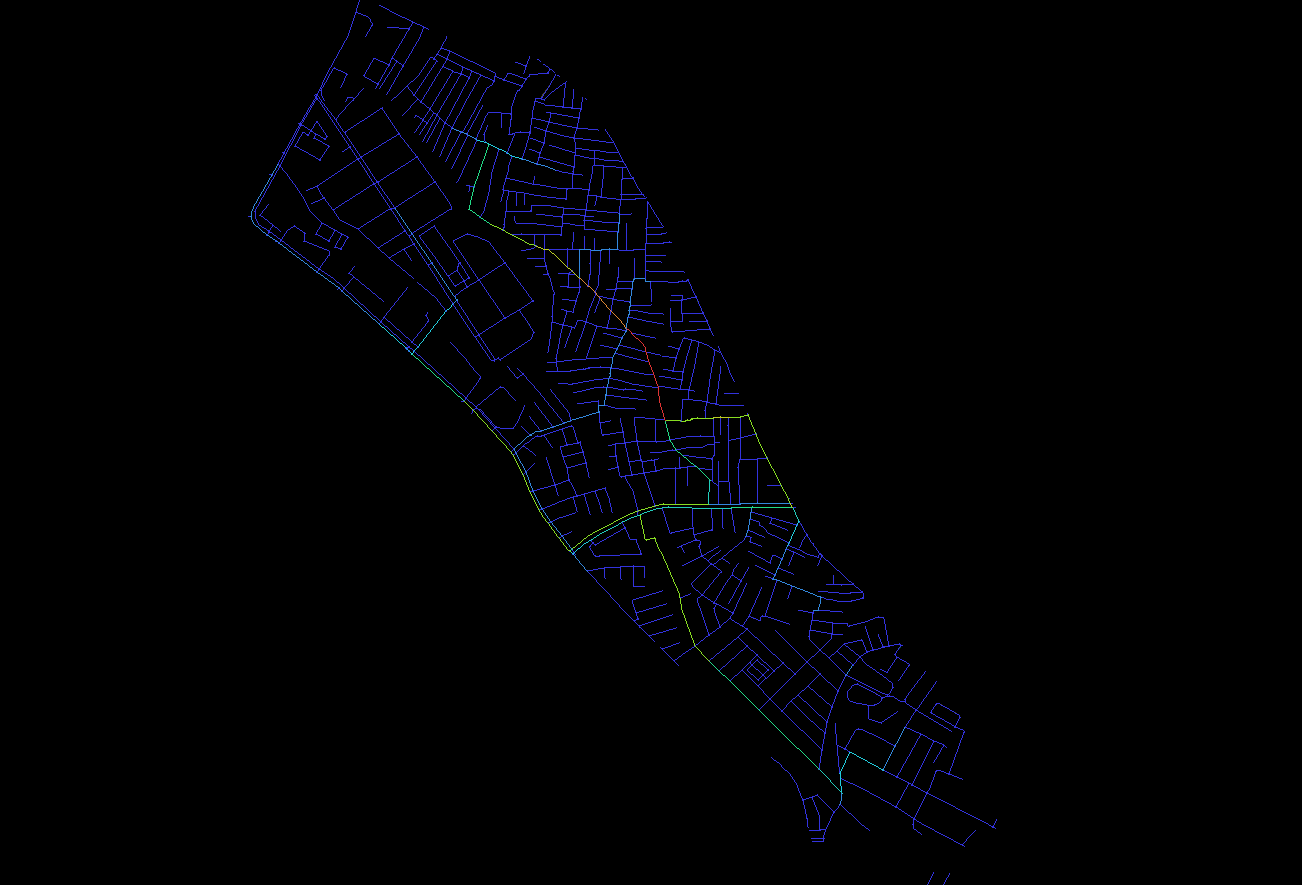
Figure 8.3:

These are roads that SSA hypothesizes are the busiest, most important roads in the network! There are also layers like T1024 Choice R100.00 metric, which will show you how the Choice measure varies with the kind of distance we set it too but since our network is rather small, these layers are pretty much the same.

8.1.5 Insights from analysis

SSA is a powerful tool to evaluate the spatial configuration of urban environments and identify potentially important streets within the network. However, it should only be used as a starting point to uncover these potentially important streets, rather than a final decision-making tool.

In order to validate the results of SSA, it is important to conduct site visits or compare the analysis with other relevant information, such as land use maps. This is because there may be other factors that influence the importance of a street beyond its spatial configuration, such as its location in relation to commercial or residential areas, the presence of important landmarks or institutions, or social and cultural factors.

For example, in the case of Map 8.3, the streets highlighted in red were identified as potentially important according to SSA. However, it was only after comparing this analysis with a land use map that it was clear that these streets were significant due to their concentration of commercial buildings and shops. In this case, the importance of the streets was related to their function within the urban environment, rather than just their spatial configuration.

Therefore, while SSA is a valuable tool for urban analysis and planning, it should always be used in conjunction with other forms of data and on-site investigation to fully understand the context and significance of potentially important streets.